Tennis Ace
- Alex Ricciardi

- Nov 20, 2020
- 13 min read
A Codecademy ‘challenging’ project from the Data Science course Machine Learning section, supervised machine learning (linear regression model).
▪ Overview:
This project is slightly different than others you can encountered on Codecademy. Instead of a step-by-step tutorial, this project contains a series of open-ended requirements which describe the project.
Project Goals: Create a linear regression model that predicts the outcome for a tennis player based on their playing habits. By analyzing and modeling the Association of Tennis Professionals (ATP) data, you will determine what it takes to be one of the best tennis players in the world.
Prerequisites: In order to complete this project, you should have completed the Linear Regression and Multiple Linear Regression lessons in the Machine Learning Course.
Using Jupyter Notebook as the project code presentation is a personal preference, not a project requirement.
▪ Project Requirements:
No three words are sweeter to hear as a tennis player than those, which indicate that a player has beaten their opponent. While you can head down to your nearest court and aim to overcome your challenger across the net without much practice, a league of professionals spends day and night, month after month practicing to be among the best in the world. Using supervised machine learning models, test the data to better understand what it takes to be an all-star tennis player.
Knowledge requirement:
Python
Python library pandas
Python library sklearn
Supervised machine learning models
▪ Links:
My Project Jupyter Notebook Python Code Presentation
Investigating the data
In the project provided file, tennis_stats.csv, is the data from the men’s professional tennis league, the ATP (Association of Tennis Professionals). Data from the top 1500 ranked players in the ATP over the span of 2009 to 2017. The statistics recorded for each player in each year include service game (offensive) statistics, return game (defensive) statistics and outcomes.
▪ Exploring the ATP data:
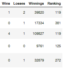
ATP DataFrame, tennis_stats, sample


ATP DataFrame Information
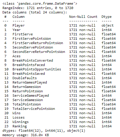
▪ Identifying the Data:
Player: name of the tennis player
Year: year data was recorded
Service Game Columns (Offensive)
Aces: number of serves by the player where the receiver does not touch the ball
DoubleFaults: number of times player missed both first and second serve attempts
FirstServe: % of first-serve attempts made
FirstServePointsWon: % of first-serve attempt points won by the player
SecondServePointsWon: % of second-serve attempt points won by the player
BreakPointsFaced: number of times where the receiver could have won service game of the player
BreakPointsSaved: % of the time the player was able to stop the receiver from winning service game when they had the chance
ServiceGamesPlayed: total number of games where the player served
ServiceGamesWon: total number of games where the player served and won
TotalServicePointsWon: % of points in games where the player served that they won
Return Game Columns (Defensive)
FirstServeReturnPointsWon: % of opponents first-serve points the player was able to win
SecondServeReturnPointsWon: % of opponents second-serve points the player was able to win
BreakPointsOpportunities: number of times where the player could have won the service game of the opponent
BreakPointsConverted: % of the time the player was able to win their opponent’s service game when they had the chance
ReturnGamesPlayed: total number of games where the player’s opponent served
ReturnGamesWon: total number of games where the player’s opponent served and the player won
ReturnPointsWon: total number of points where the player’s opponent served and the player won
TotalPointsWon: % of points won by the player
Outcomes
Wins: number of matches won in a year
Losses: number of matches lost in a year
Winnings: total winnings in USD in a year
Ranking: ranking at the end of year
Data Analysis
The project's objective is to determine what it takes to be one of the best tennis players in the world.
With that objective in mind, when using the DataFrame man_tennis, we are interested to see if strong relationships exist between some of the (Offensive) service columns values and the outcome columns values , and between some of the (Defensive) service columns values and the outcome columns values.
▪ Correlation Analysis:
The correlation coefficient is a statistical measure of the strength of the relationship between the relative movements of two variables, in our example is the pairing of the DataFrame columns to measure the strength of the relationship between two columns values. The calculated correlation values range between -1.0 and 1.0. A correlation of -1.0 shows a perfect negative correlation, while a correlation of 1.0 shows a perfect positive correlation. A correlation of 0.0 shows no linear relationship between the movement of the two variables.
Using the Pandas function DataFrame.corr(), I saved the DataFrame man_tennis columns coefficient of correlation values in a DataFrame man_tennis_corr, from it, we want to isolated the correlation coefficient values relative to the columns Wins, Winnings and Ranking to see if strong relationships exists between the (Offensive) service columns values and the outcome columns Winnings and Ranking values , and between the (Defensive) return columns values and the outcome columns Winnings and Ranking values.
Note: The pairing of the column Losses with the service and return columns is not useful to determine what it takes to be one of the best tennis players in the world. Also The correlation coefficient values relative to the Year column values is not really useful to our analysis.
DataFrame man_tennis_corr_outcome:

To refine our data analysis with the goal to determine what it takes to be one of the best tennis players in the world:
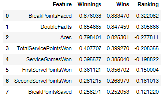
▪ I created a correlation DataFrame relative to the players serving, playing offence, using the outcomes column and pairing them with the service game columns.
DataFrame man_tennis_corr_outcome_off:
▪ I created a correlation DataFrame relative to the players receiving, playing defense, using the outcomes column and pairing them with the return game columns.
DataFrame man_tennis_corr_outcome_deff:
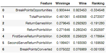
The BreakPointsOpportunities, BreakPointsFaced, DoubleFaults and Aces features seem to have strong correlations with ‘what it takes to be one of the best tennis players in the world’.
The outcome Ranking has negative correlation coefficient values relative to all the features, and the values are too low in magnitude to show a relevant correlation between the features and the Ranking outcome.
A graphical representation of the relationships between the features and the outcomes can help us visualize if linear correlations exist between some of the features and the outcomes.
▪ Features and Outcomes Relationships Graphical Visualization
To graphically visualize the relationship between the features and the outcomes, scatter plots graphs are best fitted for the task. The scatter plots graph is useful to visually identify relationships between a first and a second entries of paired data.
If it seems that the points follow a linear pattern well, a high linear correlation may exist between the paired date.
If it seems that the data do not follow a linear pattern, a no linear correlation may exist between the paired date.
If the data somewhat follow a linear path, a moderate linear correlation may exist between the paired date.
all_features_vs_outcomes_grid

Note: the 'r' represents the correlation coefficient value between a feature and an outcome.
The pairing of the outcome Ranking data with the offence and defense data seem to show that is no linear correlation between the outcome Ranking and all the features data.
The pairing of the features BreakPointsOpportunities, BreakPointsFaced, DoubleFaults and Aces data with the outcomes Winnings and Wins data seem to show a high linear correlation between the four features and the two outcomes.
Using single feature linear regression and multiple features linear regression models on the data, will help predict how those four features affect the outcomes Winnings and Wins.
Linear Regression
"In statistics, linear regression is a linear approach to modeling the relationship between a scalar response (or dependent variable) and one or more explanatory variables (or independent variables). The case of one explanatory variable is called simple linear regression. For more than one explanatory variable, the process is called multiple linear regression. This term is distinct from multivariate linear regression, where multiple correlated dependent variables are predicted, rather than a single scalar variable." Linear regression
▪ Simple Linear Regression
Simple linear regression, also called single feature linear regression in data science, is used to estimate the relationship between two quantitative variables, one independent variable and one dependent variable.
The features BreakPointsOpportunities, BreakPointsFaced, DoubleFaults and Aces showed strong correlation with the outcomes Winnings and Wins.
Winnings and Wins have very similar correlation coefficient values and scatter plots diagram results.
Understanding the data:
▪ Winnings vs Wins:
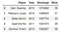
With Wins been the number of matches won in a year by the player and Winnings been the amount of US dollars won by the player in a year. Predicting Winnings will be slightly more accurate than Wins to determine ‘what it takes to be one of the best tennis players in the world’. For example, during a tournament a player that wins the tournament will have a greater amount of winnings than a player that may not have won the tournament but got second place and won more matches during the tournament.
Sam Querrey's 2010 winnings were $1,074,562 with 39 games won, verses Gilles Simon's 2012 winnings were $1,067,734 with 43 games won.
DataFrame highest_winnings:
▪ Positive features vs Negative features:
Also, when determining ‘what it takes to be one of the best tennis players in the world’ is important to understand how the features, that we want to use in our linear regression models, are correlated to the outcome Winnings relative to the player. for example: BreakPointsOpportunities and Aces are positive results relative to the player.
BreakPointsOpportunities: number of times where the player could have won the service game of the opponent
Aces: number of serves by the player where the receiver does not touch the ball
BreakPointsFaced and DoubleFaults are negative results relative to the player.
BreakPointsFaced: number of times where the receiver could have won service game of the player
DoubleFaults: number of times player missed both first and second serve attempts
I grouped the features into two categories:
Positive category: 'what the player needs to have in a significant amount, to be one of the best tennis players in the world'
Negative category: 'what the player can not to have in a significant amount, to be one of the best tennis players in the world'
▪ Positive features:
Aces: number of serves by the player where the receiver does not touch the ball
BreakPointsOpportunities: number of times where the player could have won the service game of the opponent
FirstServePointsWon: % of first-serve attempt points won by the player
SecondServePointsWon: % of second-serve attempt points won by the player
BreakPointsSaved: % of the time the player was able to stop the receiver from winning service game when they had the chance
ServiceGamesWon: total number of games where the player served and won
TotalServicePointsWon: % of points in games where the player served that they won
FirstServeReturnPointsWon: % of opponents first-serve points the player was able to win
SecondServeReturnPointsWon: % of opponents second-serve points the player was able to win
BreakPointsConverted: % of the time the player was able to win their opponent’s service game when they had the chance
ReturnGamesWon: total number of games where the player’s opponent served and the player won
ReturnPointsWon: total number of points where the player’s opponent served and the player won
TotalPointsWon: % of points won by the player
▪ Negative features:
BreakPointsFaced: number of times where the receiver could have won service game of the player
DoubleFaults: number of times player missed both first and second serve attempts
Using Real Data to predict how the features affect winnings
In the single feature linear regression models, I used the best top four correlation features to predict winnings, I used the positive features BreakPointsOpportunities and Aces data, and the negative features BreakPointsFaced, DoubleFaults data as a individual sets of variables and pair each of them with the Winnings outcome data.
best_4_features_grid:
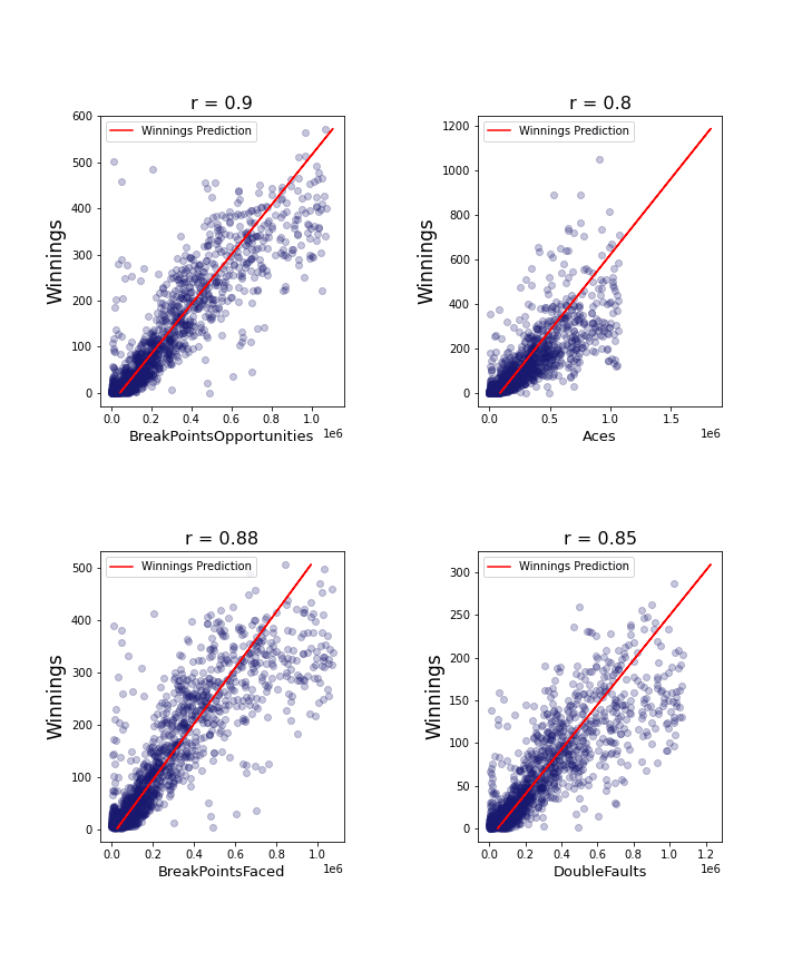
Note: the 'r' represents the correlation coefficient value between a feature and the Winnings outcome.
Base on the real data, the predicted winnings amounts increase as the values of the BreakPointsOpportunities , Aces, BreakPointsFaced and DoubleFaults features values increase.
Data Analyses Results
When determining , based on the analyses of the real data, what it takes to be one of the best tennis player in the world, we found that:
The data from ATP is composed of:
outcome results
offensive play features
defensive play features
The data reveals:
from the computed correlation coefficient between features and outcomes
from the scatter plots showing the relationship between features and outcomes
from the simple linear regression
That the best four features to understand what it takes to be one of the best tennis players in the world , are BreakPointsOpportunities , Aces, BreakPointsFaced and DoubleFaults.
And the Winnings outcome seem to be the best outcome to understand what it takes to be one of the best tennis players in the world.
We determined that relative to a player becoming the best tennis player in the world, the features BreakPointsOpportunities and Aces have a positive influence, but BreakPointsFaced and DoubleFaults have a negative influence.
In other words, a player needs to hold significant high values within the features BreakPointsOpportunities and Aces, and within the Winnings outcome,
the player also need to hold significant low values within the features BreakPointsFaced and DoubleFaults 'to be one of the best tennis players in the world'.
Machine Learning
"The purpose of machine learning is often to create a model that explains some real-world data, so that we can predict what may happen next, with different inputs. The simplest model that we can fit to data is a line. When we are trying to find a line that fits a set of data best, we are performing Linear Regression. We often want to find lines to fit data, so that we can predict unknowns." Codecademy: Introduction to Linear Regression
In Supervised learning, you train the machine using data which is well "labeled".
"Supervised machine learning algorithms are amazing tools capable of making predictions and classifications. However, it is important to ask yourself how accurate those predictions are. After all, it’s possible that every prediction your classifier makes is actually wrong! Luckily, we can leverage the fact that supervised machine learning algorithms, by definition, have a dataset of pre-labeled datapoints. In order to test the effectiveness of your algorithm, we’ll split this data into: training set, validation set and test set." Codecademy: Training Set vs Validation Set vs Test Set
▪ Simple Linear Regression
For our project we want to test how well a feature-winnings simple regression models score in predicting winnings.
We need to split our data set in training sets and test sets (real data sample).
We want to train our models using the training sets to train our models.
And score the models, how well models do at predicting winnings using the test sets.
The model scores are the models' coefficient of determination, R^2 or Score, for our example, is the coefficient of determinations of the winnings test set relative to each feature test set.
"In statistics, the coefficient of determination, is the proportion of the variance in the dependent variable that is predictable from the independent variable(s). It is a statistic used in the context of statistical models whose main purpose is either the prediction of future outcomes or the testing of hypotheses, on the basis of other related information. It provides a measure of how well observed outcomes are replicated by the model, based on the proportion of total variation of outcomes explained by the model." Coefficient of Determination
▪ Best four features
Using single feature regression models, I trained our models to predict winnings from the best four features and compare the results with the actual winnings, real data.
Results:
four_best_f_grid
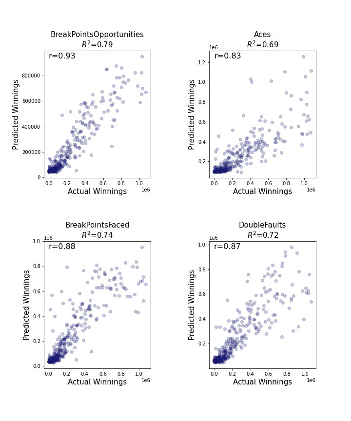
The 'r' represents the correlation coefficient value between predicted winnings and the actual winnings.
The score, 𝑅^2, represents the coefficient of determination relative to the feature test set and the winnings test set.
Note: your results will silty vary
From the the above results, we can say, with moderate certainty, that the supervised machine learning models using one of the four best features are accurate at predicting winnings.
Again, when determining ‘what it takes to be one of the best tennis players in the world’ is important to understand how the features, that we are using in our linear regression models, are correlated to the outcome Winnings relative to the player. As individual features:
- Best
BreakPointsOpportunities is the best feature a player can have in significant amount, 'to be one of the best tennis players in the world'
Aces is the second best feature a player can have in significant amount, 'to be one of the best tennis players in the world'
- Worst:
BreakPointsFaced is the worst feature for player to have, in a significant amount, 'to be an all-star tennis player'
DoubleFaults is the second worst feature a player can have, in a significant amount, 'to be an all-star tennis player'
A single feature linear regression model is good method to isolate the best features, a multiple linear regression model including two or more of the best features, may also help us to determinate ‘what it takes to be one of the best tennis players in the world’
▪ Multiple Features Linear Regression
In machine learning, the multiple linear regression models use two or more independent variables to predict the values of the dependent variable.
Four our project, it is the combinations of one or more features data, independent variables, it is used to predict winnings , the dependent variable.
For our project we want to predict winnings using two or more features combination.
For our dependent variables I used:
The Winnings outcome: number of matches won in a year.
For our independent variables I used:
- Positive two features combinations using
Aces: number of serves by the player where the receiver does not touch the ball
BreakPointsOpportunities: number of times where the player could have won the service game of the opponent
FirstServePointsWon: % of first-serve attempt points won by the player
SecondServePointsWon: % of second-serve attempt points won by the player
BreakPointsSaved: % of the time the player was able to stop the receiver from winning service game when they had the chance
ServiceGamesWon: total number of games where the player served and won
TotalServicePointsWon: % of points in games where the player served that they won
FirstServeReturnPointsWon: % of opponents first-serve points the player was able to win
SecondServeReturnPointsWon: % of opponents second-serve points the player was able to win
BreakPointsConverted: % of the time the player was able to win their opponent’s service game when they had the chance
ReturnGamesWon: total number of games where the player’s opponent served and the player won
ReturnPointsWon: total number of points where the player’s opponent served and the player won
TotalPointsWon: % of points won by the player
- Negative two features combinations using:
BreakPointsFaced: number of times where the receiver could have won service game of the player
DoubleFaults: number of times player missed both first and second serve attempts
Tow Features Regressions Results
Positive Feature: positive_two_f_grid

Note: only the two features models with a coefficient of determination values equal or superior to 0.70 have been selected.
We can also say , with moderate certainty, that the above two features combinations are the best two features combinations a player need to have in significant amount, 'to be one of the best tennis players in the world'.
Negative Feature: positive_two_f_grid
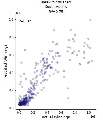
Note: only the two features models with a coefficient of determination values equal or superior to 0.70 have been selected.
We can say , with moderate certainty, that the above two features combination is the worst two features combinations a player can have in significant amount, 'to be one of the best tennis players in the world'.
Again
The 'r' represents the correlation coefficient value between predicted winnings and the actual winnings.
The score, 𝑅^2, represents the coefficient of determination relative to the multi-features test set and the winnings test set.
Note: your results can be silty vary
From the above results, we can say, with moderate certainty, that the supervised machine learning models using two features, with a coefficient of determination values equal or superior to 0.70, are accurate at predicting winnings.
Four Features Regressions Results
Note: the negative category has only two features, no negative four features combination is possible.
Positive Feature: positive_four_f_grid

Note: only the four features models with a coefficient of determination values equal or superior to 0.86 have been selected.
We can say , with good certainty, that the above four features combinations are the best four features combinations a player can have in significant amount, 'to be one of the best tennis players in the world'.
From the above results, we can say, with good certainty, that the machine supervised learning models using four features, with a coefficient of determination values equal or superior to 0.86, are accurate at predicting winnings.


Comments