Alex Ricciardi

Jan 31, 202111 min read

Viral Tweets

Updated: Feb 6, 2021

Twitter Classification Cumulative Project Part-1

My Codecademy Challenging Part-1 Project From The Data Scientist Path Foundations of Machine Learning: Supervised Learning Course, Advance Classification Models Section

▪ Overview:

In this project, Twitter Classification Cumulative Project, I use real tweets to find patterns in the way people use social media. There are two parts to this project:

Part-1: Viral Tweets (This Section).
Part-2: Classifying Tweets, using Naïve Bayes classifiers to predict whether a tweet was sent from New York City, London, or Paris.

▪ Viral Tweets Project Goal:

Predict Viral Tweets, using a K-Nearest Neighbors classifier to predict whether or not a tweet will go viral.

Note: I went beyond the project's goal, by evaluating three different models.

▪ Project Requirements:

Be familiar with:

Python3
Machine Learning: Supervised Learning
The Python Libraries:

Pandas

NumPy

Matplotlib

Sklearn

▪ Links:

Jupyter Notebook Code Presentation

Exploring The Data

▪ Number of tweets in the data: 11'099

▪ Features and features' data type:

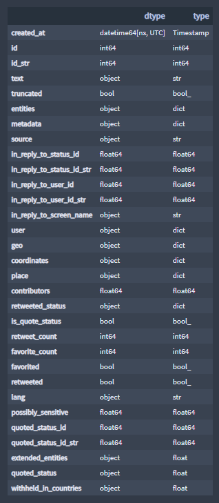
A detailed description of the features can be found in The Twitter Data Dictionary.

▪ Some features are dictionaries, for example, the feature "user" objects are dictionaries:

Sample:

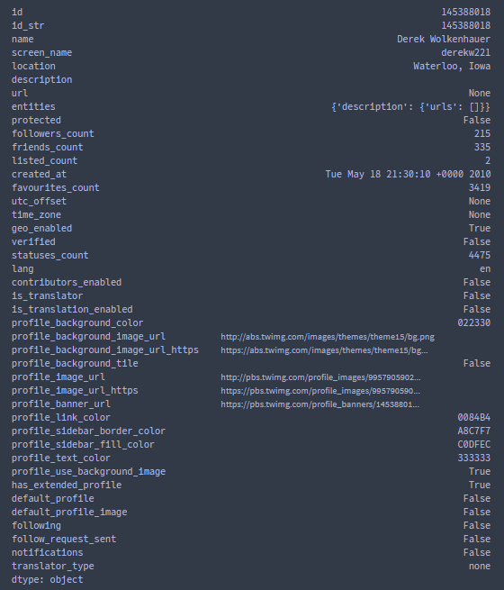
The "user" dictionary has potentially useful information to predict if a tweet will go viral.

▪ The "retweeted_status" dictionary :

Sample:

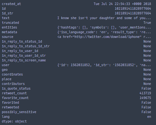
The "retweet_count" and "favorite_count" features can potentially be useful to predict if a tweet will go viral.

K-Nearest Neighbors classifier

K-Nearest Neighbors (K-NN) algorithm is used for classification or regression.

For this project, we are using K-Nearest Neighbors classifier (KNN-classifier) models, to predict whether a tweet will go viral or not.

The central idea behind the KNN-classification algorithm is that data points with similar attributes tend to fall into similar categories, in other words, the KNN-classifier uses the viral tweets' attributes to classify or predict whether a tweet will go viral or not.

Defining Viral Tweets

The Codecademy project guide suggests to set the benchmark defining a viral tweet to 5 retweets count or to the average retweets count .

A K-Nearest Neighbors classifier is a supervised machine learning algorithm, and as a result, we need to have a dataset with tagged labels. For this specific example, we need a dataset where every tweet is marked as viral or not viral. Unfortunately, this isn't a feature of the provided dataset — I created label sets.

So how to define what is a viral tweet?

A viral tweet can be defined as a post shared by a large number of people quickly. While there are no hard rules defining a viral tweet, it’s considered viral if it has hundreds of thousands of retweets, likes, and replies.

Note:

The features "quote_count" and "reply_count" can be found in The Twitter Data Dictionary and they would be helpful in defining if a tweet is a viral tweet, but unfortunately they are not part of this project provided data.

On a positive note, while exploring the provided data, the feature "favorite_count", which indicates how many times the tweet has been liked, can be found in the provided data dictionary "retweeted_status".

The feature "retweet_count" can be found as one of the main features in the provided data.

+ Exploring the feature "retweet_count"

A good place to start is to look at the number of retweets the tweet has. This can be found in the feature "retweet_count".

▪ The highest "retweet_count" value: 413'719 retweets

▪ The tweet with the highest "retweet_count" value:

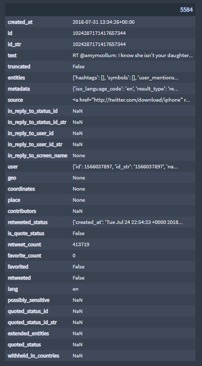
Note:

For this project, the total number of tweets provided with the data is 11'099 and the highest "retweet_count" value is 413'719.

▪ Average "retweet_count": 13

A significant difference exists between the highest "retweet_count" value and the average "retweet_count" value.

I decided to visualized the feature "retweet_count" by using scatter plots.

▪ "retweet_count" scatter plots:

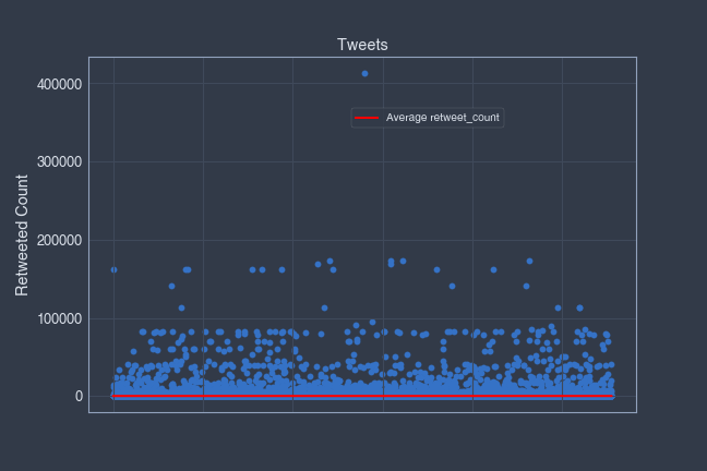
The highest "retweet_count" value is an outlier, let's remove it from the graph and try to improve the readability of the average line.

No outliner:

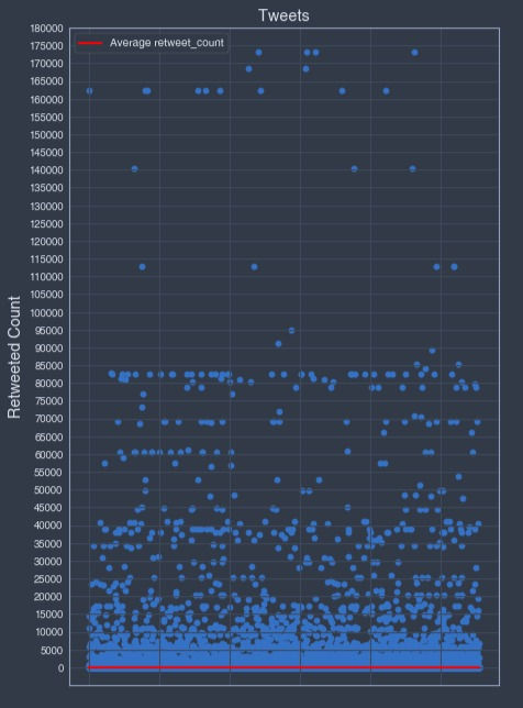
Based on the above "retweet_count" data points distribution, I decided, on top of the 5 retweets count and the average retweets viral retweet benchmarks, to add an extra benchmark at the 10'000 retweets value count.

10'000 benchmark:

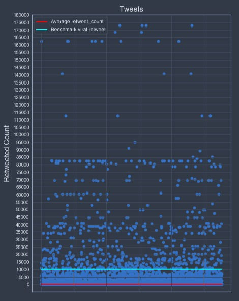
For this particular data sample, the 10'000 "retweet_count" benchmark seems to be the best fitted "retweet_count" benchmark meeting the viral tweet requirements definition.

For this project, I decided to train and evaluate three different models using the benchmarks:

5 "retweet_count" benchmark
Average "retweet_count" benchmark
10'000 "retweet_count" benchmark

+ Making Retweet Count Labels:

"is_viral_retweet_b5", 5 "retweet_count" benchmark
"is_viral_retweet_b_avg", Average "retweet_count" benchmark
"is_viral_retweet_b10000", 10'000 "retweet_count" benchmark

The retweet count labels, "is_viral_retweet_b...", purpose is to define viral retweet classes and to train the KNN classifier models.

▪ Viral retweets' classes:

0 class, is Not a viral retweet
1 class, is a viral retweet

5 "retweet_count" benchmark number of tweet by class:

1    6242
0    4857
Name: is_viral_retweet_b5, dtype: int64

Average "retweet_count" benchmark number of tweet by class:

1    5591
0    5508
Name: is_viral_retweet_bavg, dtype: int64

10'000 "retweet_count" benchmark number of tweet by class

0    10449
1      650
Name: is_viral_retweet_b10000, dtype: int64

The "is_viral_retweet_b10000" label data, with a benchmark set to 10'000 retweets count, has a significantly lower amount of 'viral retweets class' data, 650, than 'not-viral retweets class' data, 10'449.

By consequence, the provided data, the classifier model training and test label sets contain a significant more amount of 'not-viral retweets class' than 'viral retweets class'. The data is imbalanced, What Is Data Imbalance?

Imbalanced dataset occurs when one set of classes are much more than the instances of another class where the majority and minority class or classes are taken as negative and positive. In other words, data imbalance takes place when the majority classes dominate over the minority classes.

Most machine learning models assume that data is equally distributed. This results in the algorithms being more biased towards majority classes, resulting in an unequal distribution of classes within a dataset. Also, most ML Algorithms are usually designed to improve accuracy by reducing the error. So they do not take into account the balance of classes. In such cases, the predictive model developed using conventional machine learning algorithms could be biased and inaccurate.

In other words, the significant difference between the amounts of 'not-viral retweet class' and 'viral retweet class' is corrupting the "signal", the underlying pattern that you wish to learn from the data, overfitting is occurring.

+ Exploring the feature "favorite_count"

The feature "favorite_count", which indicates how many times the tweet has been, can be found in the dictionary "retweeted_status".

▪ The highest "favorite_count" value: 560'274 likes

▪ The tweet with the highest "favorite_count" value:

Note:

For this project, the total number of tweets provided with the data is 11'099 and the highest "favorite_count" value is 560'274.

▪ Average "favorite_count": 23

A significant difference exists between the highest "favorite_count" value and the average "favorite_count" value.

I decided to visualized the feature "favorite_count" by using scatter plots.

▪ "favorite_count" scatter plots:

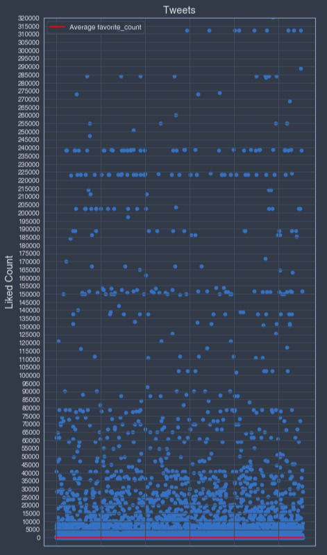
Based on the above "favorite_count" data points distribution, I decided, on top of the 5 favorites count and the average favorites viral favorite benchmarks, to add an extra benchmark at the 10'000 favorites value count.

Note: the outliners data points representing a "favorite_count" over 350'000 are not visualized in the graph above.

10'000 benchmark:

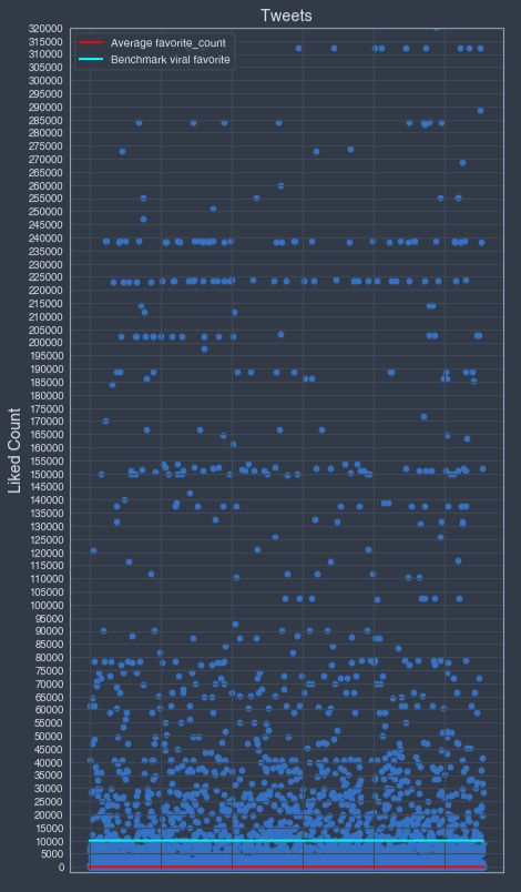
For this particular data sample, the 10'000 "favorite_count" benchmark seems to be the best fitted "favorite_count" benchmark meeting the viral tweet requirements definition.

For this project, with the "retweet_count" benchmarks, I decided to train and evaluate three different models using the benchmarks:

5 "favorite_count" benchmark
Average "favorite_count" benchmark
10'000 "favorite_count" benchmark

+ Making Favorite Count Labels:

"is_viral_favorite_b5", 5 "favorite_count" benchmark
"is_viral_favorite_b_avg", Average "favorite_count" benchmark
"is_viral_favorite_b10000", 10'000 "favorite_count" benchmark

The favorite count labels, "is_viral_favorite_b...", purpose is to define viral favorite classes and to train the KNN classifier models.

▪ Viral retweets' classes:

0 class, is Not a viral favorite
1 class, is a viral favorite

5 "favorite_count" benchmark number of tweet by class:

1    6481
0    4618
Name: is_viral_favorite_b5, dtype: int64

Average "favorite_count" benchmark number of tweet by class:

1    5581
0    5518
Name: is_viral_favorite_bavg, dtype: int64

10'000 "favorite_count" benchmark number of tweet by class:

0    9930
1    1169
Name: is_viral_favorite_b10000, dtype: int64

Similar to the "is_viral_favorite_b10000" label data, the "is_viral_favorite_b10000" label data with a benchmark set to the 10'000 favorites count, has a significantly lower amount of 'viral favorite class' data, 1'169, than the data representing 'not-viral favorite class' data, 9'930.

By consequence, the provided data, the classifier model training and test label sets contain a significant more amount of 'not-viral favorite class' than 'viral favorite class', the data is imbalanced.

In other words, the significant difference between the amounts of 'not-viral favorite class' and 'viral favorite class' is corrupting the "signal", the underlying pattern that you wish to learn from the data, overfitting is occurring.

Labels Sets

The labels sets defining viral tweet classes, are a combinations of :

- 5 count benchmark

"is_viral_retweet_b5"
"is_viral_favorite_b5"

- Average count benchmark

"is_viral_retweet_bavg"
"is_viral_favorite_bavg"

- 10'000 count benchmark

"is_viral_retweet_b10000"
"is_viral_favorite_b10000"

+ Defining the 'viral tweet label'

The viral tweet labels:

"is_viral_tweet_b5", 5 "retweet_count" and "favorite_count" benchmark
"is_viral_tweet_b_avg", Average "retweet_count" and "favorite_count" benchmark
"is_viral_tweet_b10000", 10'000 "retweet_count" and "favorite_count" benchmark

Are combinations of four classes:

[1, 1] 'is a viral tweet', 'is a viral retweet' and 'is a viral favorite'
[1, 0] 'is viral a tweet', 'is a viral retweet' and 'is not-viral a favorite'
[0, 1] 'is viral a tweet', 'is a viral favorite' and 'is not-viral a retweet'
[0, 0] 'is not-viral a tweet', 'is not-viral a retweet' and 'is not-viral a favorite'

▪ Viral tweet DataFrame sample

0        [0, 0]
1        [0, 0]
2        [0, 0]
3        [1, 1]
4        [0, 0]
          ...  
11094    [0, 0]
11095    [0, 1]
11096    [0, 0]
11097    [0, 0]
11098    [0, 0]
Name: is_viral_tweet_b10000, Length: 11099, dtype: object

Making Features

After defining the labels. I created the features data utilize to train and test the K-Nearest Neighbors (KNN) classifier models. I chose to use:

The length of the tweet.
The number followers
The friend count
The number of hashtags in the tweet.
The number of links in the tweet.
The number of words in the tweet.

+ Selected Features' Data

The data is a combination of all the selected features data, the purpose of the data is to train the KNN classifier models.

Some of the features are not part of the provided data and have to be created, other are part of the "user" dictionary.

all_tweets['tweet_length'] = all_tweets.apply(lambda tweet: len(tweet['text']), axis=1)

all_tweets['hastags_count'] = all_tweets.apply(lambda tweet: tweet['text'].count('#'), axis=1)

all_tweets['links_count'] = all_tweets.apply(lambda tweet: tweet['text'].count('http'), axis=1)

all_tweets['words_count'] = all_tweets.apply(lambda tweet: len(tweet['text'].split()), axis=1)

# The following features are found in the user dictionary
all_tweets['followers_count'] = all_tweets.apply(lambda tweet: tweet['user']['followers_count'], axis=1)

all_tweets['friends_count'] = all_tweets.apply(lambda tweet: tweet['user']['friends_count'], axis=1)

# Selected Features Data
data = all_tweets[['tweet_length','followers_count','friends_count', 'tweet_length', 'hastags_count', 'links_count', 'words_count']

Creating Training Sets And Test Sets

To split the provided data into training and test sets, I used the "train_test_split" function with the argument "random_state = 1", which sets the random seed to 1, to ensure that results are reproducible.

# 5 count benchmark
train_data_b5, test_data_b5, train_labels_b5, test_labels_b5 = 
train_test_split(data, labels_b5,  test_size = 0.2, random_state=1)

# avg count benchmark
train_data_bavg, test_data_bavg, train_labels_bavg, test_labels_bavg = train_test_split(data, labels_bavg,  test_size = 0.2, andom_state=1)

# 10000 count benchmark
train_data_b10000, test_data_b10000, train_labels_b10000, test_labels_b10000 = 
train_test_split(data,labels_b10000 , test_size = 0.2, random_state=1)

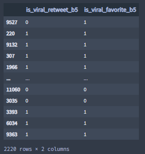
Sample "test_labels_b5":

Normalizing Select Features' Data

Many machine learning algorithms attempt to find trends in the data by comparing features of data points. However, there is an issue when the features are on drastically different scales.

Normalizing the data is the action of scaling the data.

For this exercise, the training and test data sets for each benchmark were scaled :

Sample "train_labels_b5.loc[0]":

tweet_length       140
followers_count    215
friends_count      335
tweet_length       140
hastags_count        0
links_count          0
words_count         26
Name: 0, dtype: int64

Sample "scaled_train_labels_b5[0]":

[-0.74326103 -0.02549497 -0.10028374 -0.74326103 -0.32065988  1.1246492
 -0.9627669 ]

Classifier Models

I created the KNN models with "k = 5", using the sklearn class "KNeighborsClassifier" with "n_neighbors = 5".

Next, I trained and then scored the models test sets and saved the results in a DataFrame.

The "KNeighborsClassifier.score()" returns the estimated mean accuracy on a given test data and labels.

In the other words, the accuracy score is the estimated percentage of 'viral tweet class' and 'not-viral tweet' data that the algorithm may classify correctly.

Accuracy:

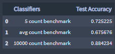
The 10000 count benchmark classifier has a higher accuracy value than the other two classifiers.

Accuracy can be an extremely misleading statistic depending on the data. When using the 10000 count benchmark classifier, like I mentioned earlier, the data is imbalance, the significant difference between the amounts of 'not-viral tweets class' and 'viral tweets class' in the provided data is corrupting the "signal", overfitting of a label class is occurring and rendering a high accuracy score.

More info: Overfitting in Machine Learning

Models Evaluations

To evaluate the models, I used the scaled test data sets to predict whether or not a tweet is a viral tweet, and compared the predicted results against the test labels sets by using the following evaluation metrics:

Accuracy
Precision
Recall

More info: 5 Classification Evaluation metrics

Predictions sample:

array([[1, 1],
       [1, 1],
       [1, 1],
       ...,
       [0, 0],
       [1, 1],
       [1, 1]])

+ Precision

Precision measures the percentage of items the classifier found that were actually relevant.

In other words, precision is the percentage of predicted 'viral retweet class' and predicted 'viral favorites class' data that was correctly classified.

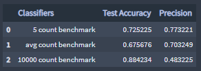
The 10000 count benchmark classifier model classified the 'viral retweet class' and the 'viral favorite class' combined data correctly 48% of the time.

+ Recall

Recall measures the percentage of the relevant items the classifier was able to successfully find.

In other words, recall is the combined percentage of predicted 'viral retweet class' and predicted 'viral favorite class' data that the classifier model successfully classify.

The 10000 count benchmark classifier has a notable lower recall score than the other two classifiers, like I mentioned earlier, the significant difference between the amounts of 'not-viral tweet class' data and ' viral tweet class' data is corrupting the "signal", the underlying pattern that you wish to learn from the data, overfitting of the label class 'not-viral tweet class' data is occurring and rendering a too low of an amount of predicted 'viral tweet class' data.

+ Test 'is a viral tweet class' vs predicted 'is a viral tweet class'

The 10000 count benchmark classifier model predicted a significantly lower amount of "Predicted Viral Tweets" than the "Test Set Viral Tweets" contain, validating the assumption that the data is imbalanced, the "signal" is weak and 'not-viral tweet class' data overfitting is occurring, when using the 10'000 benchmark with the features "retweet_count" and "favorite_count". The model is deficient at predicting a significant amount of 'viral tweet class' data.

Improving Models

The Codecademy project guide goal is to predict whether or not a tweet will go viral using a K-Nearest Neighbor classifier model, using the 5 count benchmark or the average count benchmark classifiers.

The classifiers, respectively, predict if a tweet will have 5 or more retweets or/and favorites, and if a tweet will have an average or more retweets or/and favorites.

Earlier, a real viral tweet was defined as a tweet having hundreds of thousands of retweets, likes and replies, under that definition, both classifiers are not the right models to predict whether or not a tweet will go viral.

But due to the size of the provided data (sharing files on the web size limitations), the test and training sets relative small sizes and other limiting factors, and for the sake of this exercise, a viral tweet would be best defined as a tweet with an average retweet and favorite counts.

The KNN classifier models can be improved by finding the best K value for each model. I found the best K fit for each models by initializing the model with different K values, and by training and evaluating the initialized models

I also tried to address the class imbalanced issue when using the 10000 count benchmark classifier model.

Different ways can be utilize to address imbalanced data, 5 Different Ways To Reduce Noise In An Imbalanced Dataset.

To address the imbalanced between the amounts of 'viral tweet class' data and 'not-viral tweet class' data, I tried:

to calibrate my 10000 count benchmark classifier model using the CalibratedClassifierCV from the SKlearn library, How to Calibrate Probabilities for Imbalanced Classification.
to utilize a different model, the LogisticRegression model from SKlearn library with the argument "class_weight=‘balanced’".

+ Calibrating KNN Classifier 10'000 Benchmark

Evaluation results:

Accuracy: 0.9387387387387387
Precision: 0.8333333333333334
Recall: 0.10135135135135136

The above evaluation scores are the best results that I obtained after calibrating the 10000 count benchmark classifier model.

Even if the precision has a sufficient high score the recall score is notably too low, the model is still deficient at predicting a significant amount of 'viral tweet class' data.

See code .

The provided data is just too small of a sample when using any of the KKN 10000 count benchmark models.

+ Logistic Regression Model, 10'000 count benchmark

Evaluation results:

Accuracy: 0.4783783783783784
Precision: 0.09728867623604466
Recall: 0.8243243243243243

The Logistic Regression 10000 count benchmark model with balanced classes has a better recall score value than the KNN 10000 count benchmark model but the accuracy scores is low, and the precision score value is notable too low. The model is unreliable.

+ Choosing K

The KNN classifier models were initialized with `k = 5`, but I found the best K fit for each models by initializing the model with different K values, and by training and evaluating the initialized models.

See code

▪ Visualizing best K value

- Best k for the KNN 5 count Benchmark Classifier: